Paper: Adaptive Refinement and Compression for Reduced Models

Published in Computer Methods in Applied Mechanics and Engineering

Paper Link

Introduction

Model reduction is a data-driven technique for accelerating the computation of many-query high-fidelity physics problems such as Bayesian inference and uncertainty quantification (UQ). Typically, in a model reduction setting one wants to solve a collection of PDEs of the form

where is a differential or integral operator, is a vector in an appropriate solution space, and is a parameterization of the problem. may describe anything from media of propagation to the geometry of a scene. In order to deploy reduced model reduction techniques to accelerate the task of computing many at various , one typically requires two things:

1. First, one requires an assumption of low dimensionality. That is, that the intrinsic dimension of the manifold the lie on (parameterized by ) is well approximated by some low dimensional space.
2. One has access to samples from a representative distribution to serve as training data for training.

However, in practice, ensuring that the training distribution in (2) is representative of the test distribution can be very difficult. There are a myriad of reasons for this: there are often subtle physics that can be missed while training, or the training set can be biased in some way, or maybe the underlying problem is sometimes subject to rare events -- either way, when ROMs encounter something during deployment that they have not been adequately trained for, the results can be disastrous (this is also true for data-driven machine learning techniques at large).

A Simplified Example

In this example, we consider a simple Burger's Equation shock propagating in one dimension. As we see below, the shock moves from left to right during the simulation.

Now, suppose we take the first third of this simulation and use it to train a reduced model. Such a reduced model will work quite well for the left part of the domain above, but likely once the shock moves out of the region where training data is available, we enter a dangerous no-man's land. Take a look at the resulting simulated reduced model below:

This unfortunate behavior is not surprising, once there is no longer training data to inform the physics of the shock, we just cannot expect a good result. Our work aims to provide reduced models with an efficient fallback solution for when this happens; ensuring we can still efficiently obtain high quality results without having to resort to solving the original equations. We do this by introducing two mechanisms: refinement, via vector-space sieving, and compression, via fast in-subspace PCA.

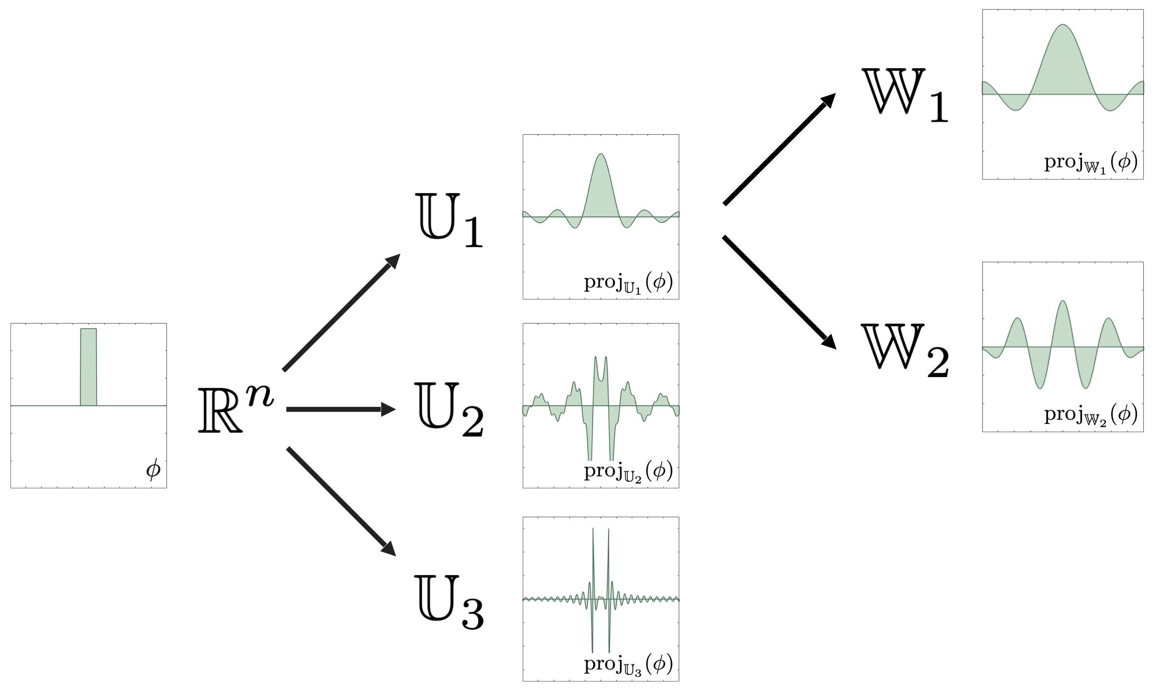
Vector-Space Sieving

The workhorse of our refinement technique is vector-space sieving. While I will not delve too deep into this topic here, the essential idea is to recursively build a hierarchical decomposition of the full-order space that the underlying physics problem resides in (say ). In our work, we build such a hierarchical decomposition from training data and the result is a refinement tree where every node of the tree corresponds to a subspace of and children of a node satisfy mutual orthogonality and sum to their parent. This gives us something that looks like the image below:

Of course, the way one chooses to decompose is ultimately up to the user. In the above image the hierarchy is built with subsequent bandpass filters. But one could just as easily recurse by slicing vectors up into disjoint domains:

Either of these two methods demonstrates the key refinement technique: we can think of any hierarchical decomposition of as a sieve (hence the name of the technique). By passing input vectors through the sieve through projection onto the children subspaces, we obtain a new set of vectors that spans a strictly larger space. Hence, reduced models after refinement will always have strictly greater model capacity than their predecessors. The crux of our technique is then to keep a separate refinement tree for each basis vector in our original reduced model. We see a representation of this below:

The final key in the technique is to use an error heuristic called dual-weighted residual error indicators,

These indicators allow us to relate the potential reduction in error (left hand side) from a refinement to potential splits in the refinement tree (right hand side). Using these error indicators as our guide, we perform refinement until we recover a good solution.

Compression

Of course, performing too many refinements also means that the dimension of our model will grow considerably. Eventually this growth will become untenable. The second half our paper focuses on a fast basis compression method meant to condense all information obtained from successive basis refinement into a smaller, more efficient basis. The key to this is performing a PCA on new data that we have acquired from online simulation. However, since we know that this new data lies in a low dimensional subspace (namely, the subspace spanned by our refined basis vectors), we can actually perform this online training extremely quickly. Indeed, suppose you have a set of training data in a low dimensional space spanned by a basis where . For a mean-zero PCA, we want to compute the singular value decomposition of

But since the range of is contained within the range of , there exists some lower dimensional (not necessarily orthogonal) such that . Recall that the left singular vectors satisfy

This is of course the same as solving

It turns out (as we show in the paper) that is it possible to keep track of the term by only performing operations of order . Furthermore, the right singular vectors (i.e., the new basis vectors) and their low dimensional coordinate representations are given by

Thus, by performing PCA on we can update our bases using new data very quickly without ever doing computations on the order of . This is the core idea behind our basis compression algorithm.

Compression therefore allows us to efficiently adapt reduced models to out-of-training distributions by supplementing the offline reduced model training with additional training that is done very efficiently online. We show in our paper that combining these two ideas leads to exciting reductions in average basis dimension over a baseline implementation of -refinement for reduced models (an alternative reduced model adaptation method that is most comparable).